Unpivot Columns in Excel🧾

Not clear about what is meant by the term "Unpivot columns", let us discuss the necessity and advantages of unpivoting the data.

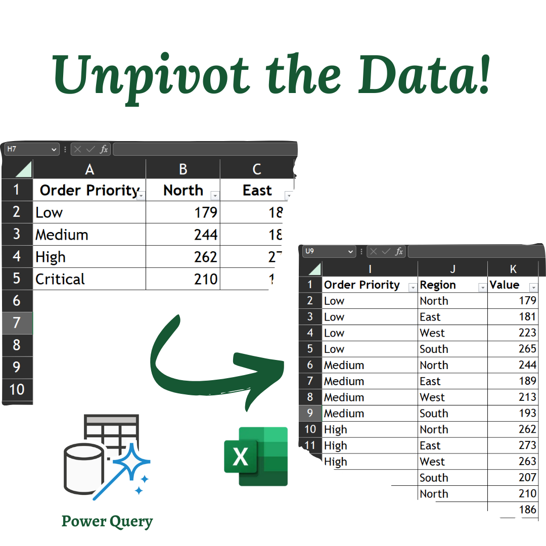
You might want to unpivot data, sometimes called flattening the data, to put it in a matrix format so that all similar values are in one column. This is necessary, for example, to create a chart or a report from the data set.

⚠️ Problem Statement

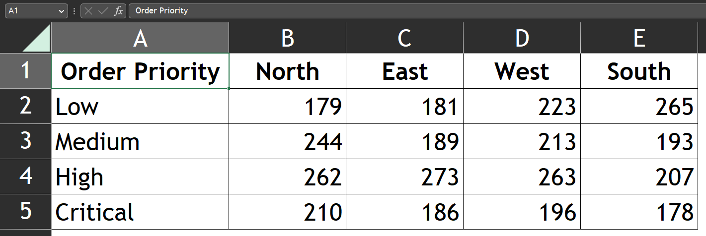
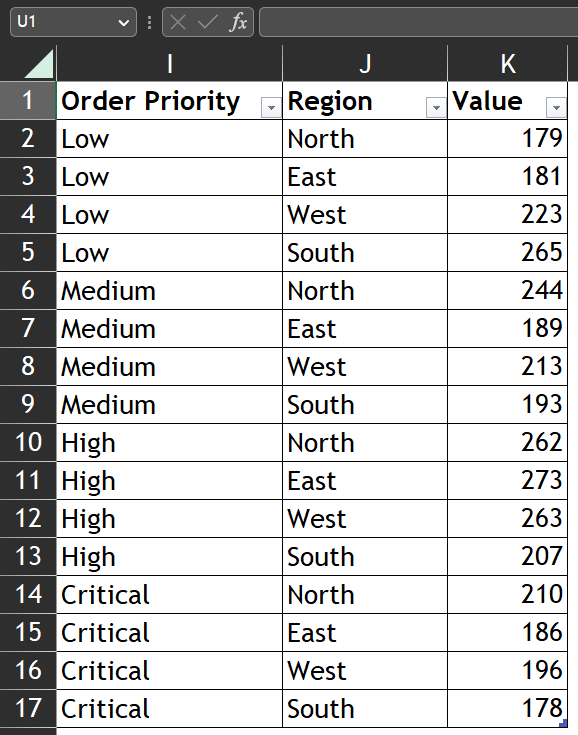
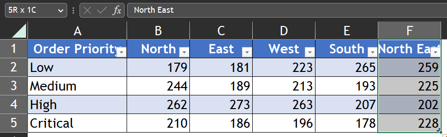
We have the region-wise sale order details with their priority level. In order to analyse this data with the help of a chart, this data won’t be useful. We have to unpivot the data and insert the column Region and flatten the data in order to create the chart.

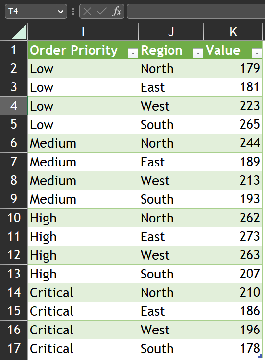
Data with us:

Data we want:

💡Solution

We can unpivot the data using Power Query Option available in the Data tab.

Steps:

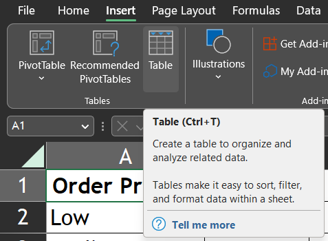
1. Convert the data into Table [Ctrl + T or using Table option in Insert tab]

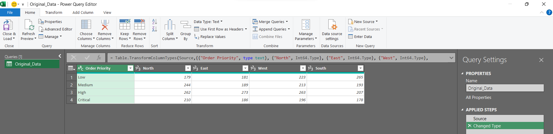
2. Rename the Table using the Table Name option in the Table Design tab (I renamed the Table to Original_Data)

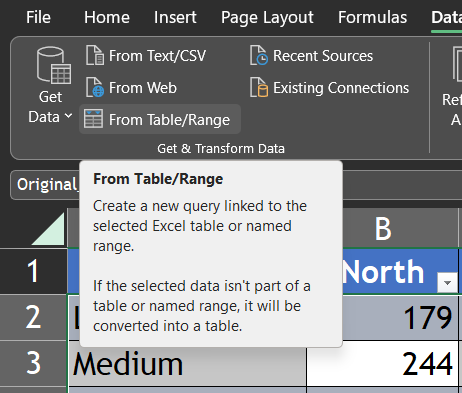
3. Navigate to the Data tab » Get & Transform Data group » From Table/Range

4. Power Query editor will be opened

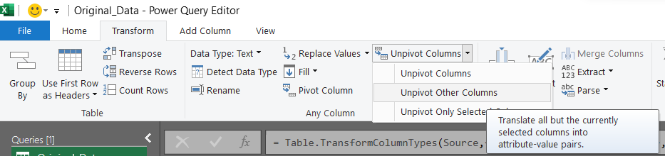
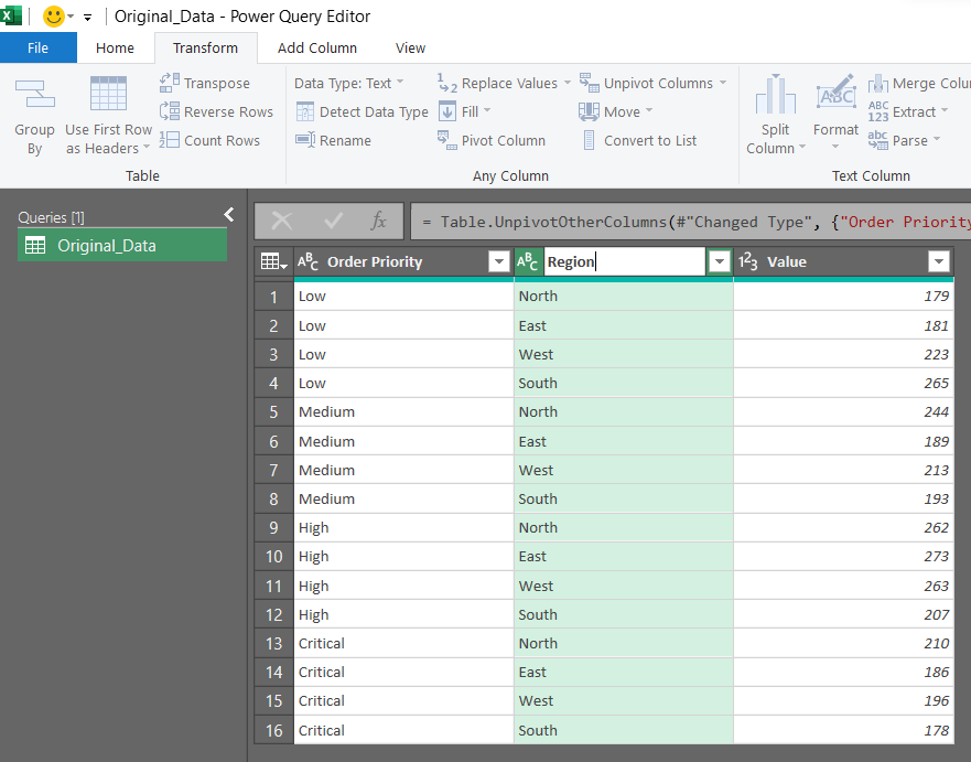
5. Navigate to the Transform tab » Any Columns group » Unpivot Columns » Unpivot other Columns.

6. Change the header 2nd column into Region

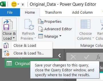
7. Navigate Home tab » Close group » Close & Load To

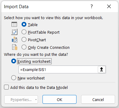
8. Choose the Location and type of data (Table).

😎 Bonus Tip (Dynamic in Nature)

Since we have loaded the data into Power query, it will be dynamic and modify itself when we add or modify any data in the original datasets.

For Instance, let us the column called North East in the Original data and see what happens when we hit refresh in the final unpivot data table.

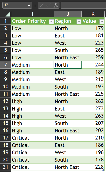
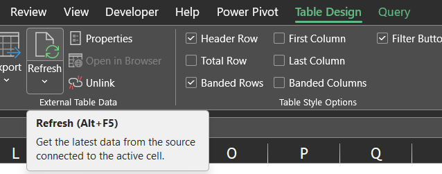
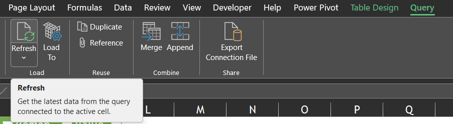
You can refresh the data by pressing Alt+F5 (or) by clicking the Refresh option available in Table Design or Query tab.

---